Rice GWAS
23 Apr 2024Today we will analyze variation in the phenotypic data. We specifically want to know if various phenotypes vary by region or population, and whether we can identify SNPs that are associated with variation in a trait of interest.
IF YOU PREFER TO WORK ON YOUR OWN COMPUTER YOU SHOULD BE ABLE TO FOR THIS LAB (with Rstudio and appropriate packages installed)
Please clone your Assignment_5 repository to find the Assignment_5_template.Rmd file to record your answers.
Goals
- Examine and summarize some of the Rice trait data
- Perform a GWAS for a trait
- Find candidate genes underlying a GWAS peak.
Reading
Nice review on GWAS procedures, including Q-Q plot from Balding, 2006. Will need library VPN.
The Wikipedia article on GWAS is pretty good.
GWAS Q & A Brookfield, 2010
Information on multiple tetsing
Load libraries
library(tidyverse)
library(statgenGWAS) #needed for GWAS
Plotting trait data
We need to get the population assignments from Admixture in the same data frame as the PCA genotype assignments and the phenotypic data. We can use a couple of the objects saved in the last lab to create what we need.
Load data from last lab
load("../../assignment_04-username/output/data_from_SNP_lab.Rdata")
You will need to change this path to the location of your data_from_SNP_lab.Rdata file
Join the data together. We will have one data frame with the PCs, the population assignments, and the phenotypes
pheno.geno.pca.pop <- left_join(geno.pca.pop, data.pheno, by=c("ID" = "NSFTVID"))

#get rid of spaces in the phenotype names with "make.names()"
colnames(pheno.geno.pca.pop) <- make.names(colnames(pheno.geno.pca.pop))

head(pheno.geno.pca.pop)
## # A tibble: 6 × 56
##   ID        PC1    PC2    PC3     PC4    PC5      PC6     PC7    PC8    PC9
##   <chr>   <dbl>  <dbl>  <dbl>   <dbl>  <dbl>    <dbl>   <dbl>  <dbl>  <dbl>
## 1 NSFTV1 -31.5   -2.15  19.2  -1.27    1.10   -0.120   0.0553 -1.85   0.221
## 2 NSFTV3  46.5   19.7    3.80  0.0722 -2.03  -14.3    -4.55   -0.145 -1.61
## 3 NSFTV4  36.8  -21.7   -2.82 -5.76    1.17   -6.17   12.0     5.34  17.7
## 4 NSFTV5  -5.56  -8.36  -2.08 40.1    -1.65   -0.361   0.654   4.78  -0.125
## 5 NSFTV6  35.0  -21.6   -3.12 -6.11    1.82   -7.02   14.1     5.88  19.7
## 6 NSFTV7 -19.4    1.85 -19.1  -0.502  -0.291   0.0578  0.882   1.07   1.11
## # ℹ 46 more variables: PC10 <dbl>, pop1 <dbl>, pop2 <dbl>, pop3 <dbl>,
## #   pop4 <dbl>, assignedPop <chr>, maxPr <dbl>, plot.order <int>,
## #   Accession_Name <chr>, Country_of_Origin <chr>, Region <chr>, Alu.Tol <dbl>,
## #   Flowering.time.at.Arkansas <dbl>, Flowering.time.at.Faridpur <dbl>,
## #   Flowering.time.at.Aberdeen <dbl>, FT.ratio.of.Arkansas.Aberdeen <dbl>,
## #   FT.ratio.of.Faridpur.Aberdeen <dbl>, Culm.habit <dbl>,
## #   Leaf.pubescence <dbl>, Flag.leaf.length <dbl>, Flag.leaf.width <dbl>, …
Check the dimensions
dim(pheno.geno.pca.pop)
## [1] 413 56
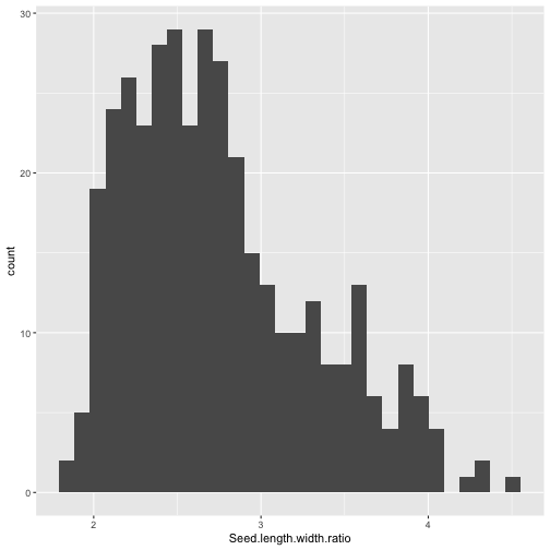
One of the defining characteristics of rice is the grain or seed shape (short, medium, or long grain). Let’s examine the distribution of seed length to width ratios. You will recall we can make a histogram as follows:
library(ggplot2)
pheno.geno.pca.pop %>%
  ggplot(aes(x=`Seed.length.width.ratio`)) +
  geom_histogram()
## Warning: Removed 36 rows containing non-finite values (`stat_bin()`).
It might be interesting to ask if the distributions look similar for different regions.
We can easily produce separate histograms for each level of a factor (as you saw in the ggplot tutorial). As a refresher, first we create a plot object, called pl, using the ggplot() function. Then we add additional information to the plot. the mapping=aes() argument tells R about the “aesthetics” of the plot, in other words which variable should be mapped to which aspect of the plot.
pl <- ggplot(data=pheno.geno.pca.pop, aes(x=Seed.length.width.ratio)) #create the basic plot object
pl <- pl + geom_histogram(binwidth=.5) #tell R that we want a histogram, with binwidth of .5
pl <- pl + facet_wrap(facets= ~ Region, ncol=3) # a separate plot ("facet") for each region, arranged in 3 columns
pl <- pl + ggtitle("Seed length width ratio") #add a title
pl #display the plot
We are a little sparse on data for faceted histograms to be a great way to visualize the results.
As you know, an alternative and useful way to display the data is to use a boxplot. The horizontal line is the median and the box is the inter-quartile range (25th to 75th percentile). See the link for more details.
Try re-plotting as a box plot.
For the rest of the lab, choose a trait to work on. I recommend one of Flowering.time.at.Aberdeen, Leaf.pubescence, Seed.length, Seed.width, Brown.rice.seed.length, Brown.rice.seed.width, Brown.rice.length.width.ratio.
Exercise 1: What Trait did you choose?
- Plot your chosen trait data using all three of these methods:
- as a single histogram for all of the data
- as separate histograms for each of the 4 population assignments made by Admixture
- as a boxplot separated by population assignments made by Admixture.
- Based on these plots do you think that your trait varies by population?
- optional Try using the “violin” geom.
Hint: you will need to use a different binwidth than I used with Seed.length.width (or don’t specify it at all and let R choose the default).
Hint: the relevant column name for population is “assignedPop”.
These plots may make you want to know the mean for your trait. Remember that we can use summarize to get a mean for each group. For example, if our trait of interest was Seed length width ratio. Also we may want to calculate the standard error of the mean. Here I define a function to do that.
sem <- function(x, na.rm=TRUE) {
  if(na.rm) x <- na.omit(x)
  sd(x)/sqrt(length(x))
}

pheno.geno.pca.pop %>% group_by(Region) %>%
  summarize(mean.seed.lw=mean(Seed.length.width.ratio,na.rm=T),
            sem.seed.lw=sem(Seed.length.width.ratio)
  ) %>%
  arrange(desc(mean.seed.lw))
## # A tibble: 10 × 3
##    Region   mean.seed.lw sem.seed.lw
##    <chr>           <dbl>       <dbl>
##  1 America          3.05      0.0678
##  2 Mid East         2.89      0.131
##  3 Pacific          2.84      0.102
##  4 S Asia           2.83      0.0666
##  5 Africa           2.79      0.0915
##  6 <NA>             2.78      0.0916
##  7 SE Asia          2.57      0.0751
##  8 C Asia           2.48      0.178
##  9 Europe           2.45      0.0762
## 10 E Asia           2.44      0.0542
For the seed length width trait, there appear to be differences in the means between regions. We can ask if these differences are significant by performing an ANOVA. More info on ANOVA.
aov1 <- aov(Seed.length.width.ratio ~ Region,data=pheno.geno.pca.pop) #1-way ANOVA for Seed.length.width.ratio by Region
summary(aov1)
The very low p-value for Region indicates that Seed length width ratio varies significantly by region.
Exercise 2:
- Obtain the mean of your trait for each of the four Admixture populations.
- Perform an ANOVA for your trait to test if it varies significantly by Admixture population. Show your code, the ANOVA output, and provide an interpretation.
- Discuss: Do your results suggest that populations structure could be a problem for GWAS for this trait?
aov2 <- aov(Seed.length.width.ratio ~ assignedPop,data=pheno.geno.pca.pop)
summary(aov2)
GWAS
A Genome Wide Association Study (GWAS) looks for significant associations between allele state at SNPs and phenotypic traits. It tests each SNP in turn.
Prepare data
statgenGWAS needs four data frames/tibbles and optional covariates:
- Genotype Data, we will call it “data.geno”, that contains the genotype data at each SNP for each individual or strain.
- Genotype Map, we will call it “data.map” that contains information on the location of each SNP (chromosome and bp). The SNP order in data.geno and data.map need to be the same
- A phenotype data frame. We will use the existing data.pheno that contains the phenotype information for each individual or line (with minor modifications).
- A Kinship matrix or “data.kinship” data frame. This indicates the pairwise genetic relatedness between individuals (statgenGWAS can estimate this matrix for us).
- Optional: A Co-variate or “data.cv” data frame. This can be used to indicate population structure, such as what we computed using Admixture or PCA analysis in the previous lab.
data.geno
Load genotype data. This is the same data you used in the last lab.
Sys.setenv(VROOM_CONNECTION_SIZE="500000") # needed because the lines in this file are _extremely_long.

data.geno <- read_csv("../../assignment_04-username/input/Rice_44K_genotypes.csv.gz", ## adjust the path to point to your assignment 4 repo
                      na=c("NA","00"))  %>%
  rename(ID=`...1`, `6_17160794` = `6_17160794...22252`) %>%
  select(-`6_17160794...22253`)
You will need to change this path to the location of your Rice_44K_genotypes.csv.gz file
statgenGWAS wants the ID info in the rownames. We can do this with:
data.geno <- data.geno %>% as.data.frame() %>% column_to_rownames("ID")
head(data.geno[,1:10])
##        1_13147 1_73192 1_74969 1_75852 1_75953 1_91016 1_146625 1_149005
## NSFTV1      TT      TT      CC      GG      TT      AA       CC       TT
## NSFTV3      CC      CC      CC      AA      GG    <NA>       CC       GG
## NSFTV4      CC      CC      CC      AA      GG      GG       CC       GG
## NSFTV5      CC      CC      TT      GG      GG      AA       TT       GG
## NSFTV6      CC      CC      CC      AA      GG      GG       CC       GG
## NSFTV7      TT      TT      CC      GG      TT      AA       CC       TT
##        1_149754 1_151492
## NSFTV1       AA       AA
## NSFTV3       TT       GG
## NSFTV4       TT       GG
## NSFTV5       TT       AA
## NSFTV6       TT       GG
## NSFTV7       AA       AA
(Note, this may take up to a minute to run)
data.map
For the data.map data frame we need an object that looks like:
##         chr   pos
## 1_13147   1 13147
## 1_73192   1 73192
## 1_74969   1 74969
## 1_75852   1 75852
## 1_75953   1 75953
## 1_91016   1 91016
Where the rownames are the SNP name, and there is a column for chromosome and position. Remember that the SNP names are simply chromosome and position (SNP 1_13147 is on chromosome 1 at basepair position 13147)
Exercise 3: Complete the code below to generate a data.map object like the one above. Note that “chr” and “pos” should be numeric.
Hint: Look at help for the separate command. You will need to specify the into, sep, convert and remove arguments.
First create the object. You do not need to modify this block
# This is one of the rare cases where tibbles and data frames are not interchangeable
# This is because we need to have rownames and tibbles do not allow rownames
# So be sure to used "data.frame()" rather than "tibble()"

data.map <- data.frame(SNP=colnames(data.geno)) # create the object
head(data.map) # take a look
Now use separate to create the chr and pos columns. You need to modify this block:
data.map <- data.map %>%
  separate(SNP, <FILL THIS IN> ) %>%
  column_to_rownames("SNP")

head(data.map) # check to make sure it looks correct
Note It is very important that the pos column is either class integer or numeric. Do you remember how to check that the column is considered an integer or numeric and change it if not?
Hint: Think about the as.numeric() function or the convert argument in separate.
data.pheno
Here we need to make four changes to our data.pheno data frame:
- rename the “NSFTVID” column to “genotype”
- only keep numeric columns
- convert from a tibble to a data frame.
- fix the column names to remove spaces
data.pheno.small <- data.pheno %>%
  set_names(make.names(colnames(.))) %>% # fixes the names
  rename(genotype=NSFTVID) %>%
  select(genotype, where(is.numeric)) %>%
  as.data.frame()

head(data.pheno.small)
##   genotype Alu.Tol Flowering.time.at.Arkansas Flowering.time.at.Faridpur
## 1   NSFTV1    0.73                   75.08333                         64
## 2   NSFTV3    0.30                   89.50000                         66
## 3   NSFTV4    0.54                   94.50000                         67
## 4   NSFTV5    0.44                   87.50000                         70
## 5   NSFTV6    0.57                   89.08333                         73
## 6   NSFTV7    0.86                  105.00000                         NA
##   Flowering.time.at.Aberdeen FT.ratio.of.Arkansas.Aberdeen
## 1                         81                     0.9269547
## 2                         83                     1.0783133
## 3                         93                     1.0161290
## 4                        108                     0.8101852
## 5                        101                     0.8820132
## 6                        158                     0.6645570
##   FT.ratio.of.Faridpur.Aberdeen Culm.habit Leaf.pubescence Flag.leaf.length
## 1                     0.7901235        4.0               1         28.37500
## 2                     0.7951807        7.5               0         39.00833
## 3                     0.7204301        6.0               1         27.68333
## 4                     0.6481481        3.5               1         30.41667
## 5                     0.7227723        6.0               1         36.90833
## 6                            NA        3.0               1         36.99000
##   Flag.leaf.width Awn.presence Panicle.number.per.plant Plant.height
## 1       1.2833333            0                 3.068053     110.9167
## 2       1.0000000            0                 4.051785     143.5000
## 3       1.5166667            0                 3.124565     128.0833
## 4       0.8916667            0                 3.697178     153.7500
## 5       1.7500000            0                 2.857428     148.3333
## 6       1.5500000            1                 2.859021     119.6000
##   Panicle.length Primary.panicle.branch.number Seed.number.per.panicle
## 1       20.48182                      9.272727                4.785975
## 2       26.83333                      9.166667                4.439706
## 3       23.53333                      8.666667                5.079709
## 4       28.96364                      6.363636                4.523960
## 5       30.91667                     11.166667                5.538646
## 6       24.62500                     13.333333                5.338019
##   Florets.per.panicle Panicle.fertility Seed.length Seed.width Seed.volume
## 1            4.914658             0.879    8.064117   3.685183    2.587448
## 2            4.727388             0.750    7.705383   2.951458    2.111145
## 3            5.146437             0.935    8.237575   2.926367    2.154759
## 4            4.730921             0.813    9.709375   2.382100    1.940221
## 5            5.676468             0.871    7.118183   3.281892    2.202360
## 6            5.435903             0.907    7.347255   2.528891    1.774465
##   Seed.surface.area Brown.rice.seed.length Brown.rice.seed.width
## 1          3.914120               5.794542              3.113958
## 2          3.658709               5.603658              2.566450
## 3          3.713856               6.120342              2.466983
## 4          3.700054               7.089883              2.044608
## 5          3.657370               5.136483              2.803858
## 6          3.474791               5.485345              2.188882
##   Brown.rice.surface.area Brown.rice.volume Seed.length.width.ratio
## 1                3.511152          7.737358                   2.188
## 2                3.287373          5.105350                   2.611
## 3                3.334126          5.126958                   2.815
## 4                3.297792          4.085133                   4.076
## 5                3.284328          5.555183                   2.169
## 6                3.101569          3.591045                   2.905
##   Brown.rice.length.width.ratio Straighthead.suseptability Blast.resistance
## 1                         1.861                   4.833333                8
## 2                         2.183                   7.831667                4
## 3                         2.481                         NA                3
## 4                         3.468                   8.333333                5
## 5                         1.832                   8.166667                3
## 6                         2.506                   8.585000                2
##   Amylose.content Alkali.spreading.value Protein.content
## 1        15.61333               6.083333            8.45
## 2        23.26000               5.638889            9.20
## 3        23.12000               5.527778            8.00
## 4        19.32333               6.027778            9.60
## 5        23.24000               5.444444            8.50
## 6        20.18667               6.000000           11.75
data.cv
Here we make a dataframe of possible covariates
data.cv <- geno.pca.pop %>%
  as.data.frame() %>%
  column_to_rownames("ID")
create the gdata object
To run statgenGWAS we bring data.geno, data.map, data.pheno, and data.cv together into a single object gData.rice
gData.rice <- createGData(geno=data.geno, map = data.map, pheno = data.pheno.small, covar = data.cv)
Note If you ran into an error, is your pos column numeric?
recode the genotypes
statgenGWAS needs the genotypes to be numeric, and we also need to remove redundant (identical) SNPs and replace missing values. Luckily statgen has a function that does all of this for us.
There are various methods to replace missing values. Overall the process is called “imputing” and at its best imputing uses existing information to make an educated guess about the most likely value. That process takes a long time and so here we will just put in a random value based on the allele frequency at the SNP with missing info. This will take a minute or so to run.
set.seed(123)
gData.rice.recode <- gData.rice %>% codeMarkers(verbose = TRUE)
## Input contains 36900 SNPs for 413 genotypes.
## 0 genotypes removed because proportion of missing values larger than or equal to 1.
## 0 SNPs removed because proportion of missing values larger than or equal to 1.
## 569 duplicate SNPs removed.
## 660509 missing values imputed.
## 454 duplicate SNPs removed after imputation.
## Output contains 35877 SNPs for 413 genotypes.
data.kinship
A Kinship matrix is one way to adjust for population structure. Kinship refers to the genetic relatedness between individuals. For example, if you have siblings your kinship with them is 50%. Similarly your kinship with each of your parents is 50%.
Since we do not know the pedigree of these rice strains, we can instead determine kinship from the observed genotypic data. The kinship function calculates this for us.
data.kinship <- kinship(gData.rice.recode$markers)
Run the GWAS
We will compare GWAS run with a few different population structure corrections and methods
- No correction
- Population PCAs as covariate
- Kinship matrix as correction
Run the code below, replacing TRAIT with the name of your trait.
No correction
To see what the GWAS looks like with no correction we will give statgenGWAS a matrix filled with zeros.
#define our zero matrix
nullmat <- matrix(0, ncol=413,nrow=413, dimnames = dimnames(data.kinship))

# run the GWAS
gwas.noCorrection<- runSingleTraitGwas(gData = gData.rice.recode,
                                       traits = "TRAIT",
                                       kin = nullmat)
We can get a quick summary with:
summary(gwas.noCorrection)
We can look at the Q-Q plot with:
plot(gwas.noCorrection, plotType = "qq")
And a Manhattan plot with:
plot(gwas.noCorrection, plotType = "manhattan")
In the Manhattan plot, each dot is a SNP. SNPs in red are above the significance threshold. If you see a lot of red, then that means that many, many SNPs were significant.
PCA as population correction
Let’s see if things improve if we correct for population structure. One methods is to include the PCs as co-variates in the analysis. You can this with:
# run the GWAS
gwas.PCA <- runSingleTraitGwas(gData = gData.rice.recode,
                               traits = "TRAIT",
                               kin = nullmat,
                               covar = c("PC1", "PC2", "PC3", "PC4")

)
Again, you can summarize and plot with:
summary(gwas.PCA)

plot(gwas.PCA, plotType = "qq")

plot(gwas.PCA, plotType = "manhattan")
Kinship Matrix
An alternative strategy for population structure correction is to use a kinship matrix, which provides the genetic relatedness of each strain to all of the others.
# run the GWAS
gwas.K <- runSingleTraitGwas(gData = gData.rice.recode,
                             traits = "TRAIT",
                             kin = data.kinship)
summary(gwas.K)

plot(gwas.K, plotType = "qq")

plot(gwas.K, plotType = "manhattan")
Exercise 4: Compare the Q-Q and Manhattan plots of the no correction, PCA correction, and kinship matrix runs. Based on the no-correction results, do you think a correction was needed? Did the corrections make a difference? If so, which one worked better? How did this effect the number of “significant” SNPs in the Manhattan plot? (In the Manhattan plot the horizontal line represents the significance threshold. If you don’t see any dots above the line, nothing was).
get the significant SNPs
Let’s retrieve the significant SNPs for our trait. Choose which ever model you think was best, and then extract the SNPs with:
sigSnps <- gwas.K$signSnp[[1]]
sigSnps
In this table, some of the column names should be obvious. Here are some of the others:
- allFreq: the minor allele frequency at that SNP
- effect: the change in the trait value associated with the SNP
- effectSE: the standard error of the estimated effect
- RLR2: likelihood-ratio-based R2 as defined in Sun et al. (2010)
- LOD: -log10(P) (which isn’t a true LOD score…)
- propSnpVar: of the total variance in the trait, what proportion is “explained” by this SNP
Exercise 5:
A) Sort the significant SNPs to find the most significant ones (smallest pValue).
Hint: Think back to tidyverse if you don’t remember how to arrange a data frame.
B) Look for genes close to the most significant SNP using the rice genome browser. Pick a significant SNP from your analysis and enter its chromosome and position in the search box. The browser wants you to enter a start and stop position, so for example, you should enter “Chr3:30449857..30449857” and then choose “show 20kb” from the pulldown menu on the right hand side. Report the SNP you chose and the three closest genes. These are candidate genes for determining the phenotype of your trait of interest in the rice population. Briefly discuss these genes as possible candidates for the GWAS peak. Include a Screenshot of the genome browser in your answer
Hint: You can take a screenshot on your JetStream instance by clicking on the app-chooser (bottom left, many small tiles) and searching for “screenshot”
Hint: You can include an image in your knitted Rmd file with  on its own line, where MyImage.jpg is the path to your image.